17 Algorithms Machine Learning Engineers Need to Know
Introduction
Machine learning is a technique that allows computers to use existing data to forecast future behaviors, outcomes, and trends. Using machine learning, computers learn without being explicitly programmed.
Quick Snapshot
Flavors of Machine Learning
Machine learning uses two types of techniques: supervised learning, which trains a model on known input and output data so that it can predict future outputs, and unsupervised learning, which finds hidden patterns or intrinsic structures in input data.

A supervised learning algorithm takes a known set of input data and known responses to the data (output) and trains a model to generate reasonable predictions for the response to new data. Supervised learning uses classification and regression techniques to develop predictive models.
- Classification techniques predict categorical responses, for example, whether an email is genuine or spam, or whether a tumor is cancerous or benign. Classification models classify input data into categories. Typical applications include medical imaging, image and speech recognition, and credit scoring.
- Regression techniques predict continuous responses, for example, changes in temperature or fluctuations in power demand. Typical applications include electricity load forecasting and algorithmic trading.
Unsupervised learning finds hidden patterns or intrinsic structures in data. It is used to draw inferences from datasets consisting of input data without labeled responses.
- Clustering is the most common unsupervised learning technique. It is used for exploratory data analysis to find hidden patterns or groupings in data.
Choosing the right algorithm
Finding the right algorithm is partly based on trial and error even highly experienced data scientists cannot tell whether an algorithm will work without trying it out. Highly flexible models tend to overfit data by modeling minor variations that could be noise. Simple models are easier to interpret but might have lower accuracy. Therefore, choosing the right algorithm requires trading off one benefit against another, including model speed, accuracy, and complexity.
With this context, presenting the listing of algorithms collated from different sources.I hope this finds you interesting & useful.
If you have questions, please do leave your questions in the comments section.

Here are the details of each algorithm :
- Support vector machines find the boundary that separates classes by as wide a margin as possible. When the two classes can’t be clearly separated, the algorithms find the best boundary they can.It is able to run fairly quickly. Where it really shines is with feature-intense data, like text or genomic. In these cases, SVMs are able to separate classes more quickly and with less overfitting than most other algorithms, in addition to requiring only a modest amount of memory.

Image – Support Vector Machines - Discriminant Analysis is a supervised learning technique that can be used for classifying numerical variables in conjunction with a single categorical target. The method is useful for feature selection because it identifies the combination of features or parameters that best separates the groups.
Image – Discriminant analysis - Bayesian methods have a highly desirable quality: they avoid overfitting. They do this by making some assumptions beforehand about the likely distribution of the answer. Another byproduct of this approach is that they have very few parameters.
- Nearest Neighbor algorithm is a method for classifying objects based on the closest training examples in the feature space. Nearest Neighbor is a type of instance-based learning or lazy learning where the function is only approximated locally and all computation is deferred until classification.
- Neural networks and perceptrons Neural networks are brain-inspired learning algorithms covering multiclass, two-class, and regression problems. input features are passed forward (never backward) through a sequence of layers before being turned into outputs. In each layer, inputs are weighted in various combinations, summed, and passed on to the next layer. This combination of simple calculations results in the ability to learn sophisticated class boundaries and data trends, seemingly by magic. Many-layered networks of this sort perform the “deep learning” that fuels so much tech reporting and science fiction.
Image – Neural networks Check out compilation on Data Science, Machine Learning, and Artificial Intelligence courses that will help boost your career and expand your knowledge.
- Linear regression fits a line (or plane, or hyperplane) to the data set. It’s a workhorse, simple and fast, but it may be overly simplistic for some problems.
Image – Linear regression / Source – Azure - The Support Vector Regression (SVR) uses the same principles as the SVM for classification, with only a few minor differences. First of all, because the output is a real number it becomes very difficult to predict the information at hand, which has infinite possibilities. In the case of regression, a margin of tolerance (epsilon) is set in approximation to the SVM which would have already requested from the problem. But besides this fact, there is also a more complicated reason, the algorithm is more complicated therefore to be taken in consideration.
- Gaussian Process Regression (GPR) provides a different way of characterizing functions that does not require committing to a particular function class, but instead to the relation that different points on the function have to each other.It can be used to characterize parameterized functions as a special case, but offers much more flexibility.
- Ensemble methods is basically to combine the predictions of several base estimators built with a given learning algorithm in order to improve generalizability/robustness over a single estimator.Two families of ensemble methods are usually distinguished:
-
In averaging methods, the driving principle is to build several estimators independently and then to average their predictions. On average, the combined estimator is usually better than any of the single base estimator because its variance is reduced.
-
By contrast, in boosting methods, base estimators are built sequentially and one tries to reduce the bias of the combined estimator. The motivation is to combine several weak models to produce a powerful ensemble.
-
- Logistic regression is actually a powerful tool for two-class and multiclass classification. It’s fast and simple. The fact that it uses an ‘S’-shaped curve instead of a straight line makes it a natural fit for dividing data into groups. Logistic regression gives linear class boundaries, so when you use it, make sure a linear approximation is something you can live with.
Image – Logistic regression / Source – Azure - Trees, forests, and jungles Decision forests (regression, two-class, and multiclass), decision jungles (two-class and multiclass), and boosted decision trees (regression and two-class) are all based on decision trees, a foundational machine learning concept. There are many variants of decision trees, but they all do the same thing subdivide the feature space into regions with mostly the same label. These can be regions of the consistent category or of constant value, depending on whether you are doing classification or regression.
Image – Decision tree - Clustering algorithms: Clustering can be considered the most important unsupervised learning problem; so, as every other problem of this kind, it deals with finding a structure in a collection of unlabeled data.
A loose definition of clustering could be “the process of organizing objects into groups whose members are similar in some way”. A cluster is, therefore, a collection of objects which are “similar” between them and are “dissimilar” to the objects belonging to other clusters.
We can show this with a simple graphical example:Image- Clustering algorithms (example) Source :https://home.deib.polimi.it - Clustering algorithms (K-Means) k-means clustering is a method of vector quantization that is popular for cluster analysis in data mining. k-means clustering aims to partition n observations into k clusters in which each observation belongs to the cluster with the nearest mean, serving as a prototype of the cluster. This results in a partitioning of the data space into Voronoi cells.The most common algorithm uses an iterative refinement technique. Due to its ubiquity, it is often called the k-means algorithm; it is also referred to as Lloyd’s algorithm.
Image – Convergence of k-means / Source -wikipedia - Hierarchical clustering Given a set of N items to be clustered, and an N*N distance (or similarity) matrix, the basic process of hierarchical clustering
- Start by assigning each item to a cluster, so that if you have N items, you now have N clusters, each containing just one item. Let the distances (similarities) between the clusters the same as the distances (similarities) between the items they contain.
- Find the closest (most similar) pair of clusters and merge them into a single cluster, so that now you have one cluster less.
- Compute distances (similarities) between the new cluster and each of the old clusters.
- Repeat steps 2 and 3 until all items are clustered into a single cluster of size N. (*)
Step 3 can be done in different ways, which is what distinguishes single-linkage from complete-linkage and average-linkage clustering.
This kind of hierarchical clustering is called agglomerative because it merges clusters iteratively. There is also a divisive hierarchical clustering which does the reverse by starting with all objects in one cluster and subdividing them into smaller pieces. Divisive methods are not generally available, and rarely have been applied. - Fuzzy c-means (FCM) is a method of clustering which allows one piece of data to belong to two or more clusters. This method is frequently used in pattern recognition. It is based on the minimization of the following objective function:
Image – Fuzzy C-Means Clustering function / Source : Fuzzy C-Means Clustering - Clustering as a Mixture of Gaussians There’s another way to deal with clustering problems: a model-based approach, which consists in using certain models for clusters and attempting to optimize the fit between the data and the model.
In practice, each cluster can be mathematically represented by a parametric distribution, like a Gaussian (continuous) or a Poisson (discrete). The entire data set is therefore modeled by a mixture of these distributions. An individual distribution used to model a specific cluster is often referred to as a component distribution.
A mixture model with high likelihood tends to have the following traits:
- component distributions have high “peaks” (data in one cluster are tight);
- the mixture model “covers” the data well (dominant patterns in the data are captured by component distributions).
Image -Mixture of Gaussians / Source : https://home.deib.polimi.it Check out 25 Most Popular Machine Learning Courses on Udemy that will help boost your career and expand your knowledge.
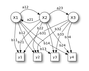
- Hidden Markov Model (HMM) is a statistical Markov model in which the system being modeled is assumed to be a Markov process with unobserved (i.e. hidden) states.A hidden Markov model can be considered a generalization of a mixture model where the hidden variables (or latent variables), which control the mixture component to be selected for each observation, are related through a Markov process rather than independent of each other. The Hidden Markov Model (HMM) is a variant of a finite state machine having a set of hidden states, Q, an output alphabet (observations), O, transition probabilities, A, output (emission) probabilities, B, and initial state probabilities, Π. The current state is not observable. Instead, each state produces an output with a certain probability (B). Usually the states, Q, and outputs, O, are understood, so an HMM is said to be a triple, ( A, B, Π ).
Image – Hidden Markov Models / Source http://www.shokhirev.com


I hope, I have covered all 3 sets of algorithms at length. If you’ve liked the post, please share it.
Useful Resources :
Additional Resources
- Curated Python Course Collection
- Python programming courses from Coursera
- Data Analysis with Python – This course will take you from the basics of Python to exploring many different types of data. You will learn how to prepare data for analysis, perform simple statistical analysis, create meaningful data visualizations, predict future trends from data, and more! Topics covered: 1) Importing Datasets 2) Cleaning the Data 3) Data frame manipulation 4) Summarizing the Data 5) Building machine learning Regression models 6) Building data pipelines Data Analysis with Python will be delivered through lecture, lab, and assignments.
- Data Processing Using Python – This course is mainly for non-computer majors. It starts with the basic syntax of Python, to how to acquire data in Python locally and from network, to how to present data, then to how to conduct basic and advanced statistic analysis and visualization of data, and finally to how to design a simple GUI to present and process data, advancing level by level.
- Data Visualization with Python – This course is to teach you how to take data that at first glance has little meaning and present that data in a form that makes sense to people. Various techniques have been developed for presenting data visually but in this course, we will be using several data visualization libraries in Python, namely Matplotlib, Seaborn, and Folium.
- Python Data Analysis – This course will continue the introduction to Python programming that started with Python Programming Essentials and Python Data Representations. We’ll learn about reading, storing, and processing tabular data, which are common tasks. We will also teach you about CSV files and Python’s support for reading and writing them.
- Python Data Visualization – This if the final course in the specialization which builds upon the knowledge learned in Python Programming Essentials, Python Data Representations, and Python Data Analysis. We will learn how to install external packages for use within Python, acquire data from sources on the Web, and then we will clean, process, analyze, and visualize that data. This course will combine the skills learned throughout the specialization to enable you to write interesting, practical, and useful programs. By the end of the course, you will be comfortable installing Python packages, analyzing existing data, and generating visualizations of that data.
- ULTIMATE GUIDE to Coursera Specializations That Will Make Your Career Better (Over 100+ Specializations covered)
References :
- Clustering algorithms
- Hidden Markov Models
- Azure ML Studio Machine Learning Algorithms
Summary
Article Name
17 Algorithms Machine Learning Engineers Need to Know
DescriptionFinding the right algorithm is partly based on trial and error even highly experienced data scientists cannot tell whether an algorithm will work without trying it out. Check out 17 Algorithms that make your life easy.
Author
Karthik
Publisher Name
Upnxtblog
Publisher Logo

More Stories
How AI is Transforming the Hiring Process in 2025
Recruitment in 2025 looks drastically different from just a few years ago. Remote work, talent shortages, and the need for...
AI and Predictive Marketing: Reaching the Right Audience at the Right Time
You’ve been targeting people, developing interesting content and managing marketing campaigns. However, it appears that your attempts are failing to...
How AI Enhances Photoshop Workflow: A Beginner’s Guide
The integration of artificial intelligence into graphic design through tools like Adobe Photoshop can save time and reduce tedious tasks,...
Innovators in Crypto: Prominent AI-Powered Coins
The cryptocurrency industry is being reshaped by the fusion of blockchain technology and artificial intelligence (AI), opening the door for...
Top AI Design Tools Every Graphic Designer Should Use in 2024
Introduction Artificial Intelligence (AI) has also found its relevance in graphic design and is quickly emerging as an effective game-changer....
Transforming Industries: The Integration of AI and Blockchain
Imagine a world where the brilliance of Artificial Intelligence (AI) meets the unbreakable security of Blockchain. This powerful convergence is...
Average Rating